Introduction

Vawtrak is a sophisticated banking Trojan that exists since 2007 and is responsible for multi million dollar damages. Since the end of October 2014, I was in control of a former Command-and-Control (C&C) server IP-address and have been capturing around 60 GB traffic for a duration of ten months from nearly 10.000 unique bots.

The results of the project showed that most of the bots were from the United States, Germany and Saudi Arabia and that most were using Windows 7 and the Internet Explorer.

A good goal would be here to disinfect the clients from the malware. Legally this could become a problem because we would have to run commands on the clients. This was technically possible and implemented already but I did not want to take the risk. Multiple contact attempts to local authorities through the university or during conferences were not answered by authorities. Or they did not want to believe. So a different approach was needed here to help these people.

The following approach was found then: As long as my sinkhole-server was responding to the malware requests, the malware will not try to contact any of the other servers in the server list. This meant that we could disinfect these bots by simply not letting them connect to the real C&C. A 200 OK from the web-server was enough to stop them connecting other C&Cs.

By implementing this approach, there were more disinfections than infections which shows the decline of the total size over time.

This article will only talk about the modelling, implementation and the results of the project.

Getting the Sinkhole

A VPS is a virtual machine running on a host which allows to run a guest operating system separated from the host. On October 2014 I acquired a Linux VPS from a Russian host in Saint Petersburg and I noticed slow network performance on the first days but that was expected due to the location.

After installing a HTTP server, unusual HTTP-request were noticed in the log files. These requests show a common pattern and repeat multiple times a second from different source addresses.

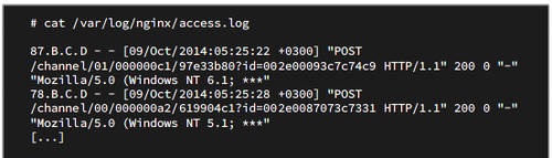Nginx logs showing bot requests

The next day the VPS was not accessible by SSH and not responding in any other form. An email from the hoster was in my inbox stating that my VPS was shut down because it was allegedly running a C&C server.

Subject: Your VPS is suspended:  Botnet controller
 Hello!
 Your VPS is suspended, we detect Vawtrack botnet controller 
 on your VPS. Let us know if you are willing to fix this.
 Thank you.

The first emal from the hoster

I asked him to proof his claims. In his following answer he gave me the information which showed that the IP-address was previously used by a C&C server. Describing him the situation that I just had the server for some days, he activated my VPS again and offered me some month of service for free.

And what about this info?
Vawtrak botnet controller located at 94.242.57.187 on port 80
(using HTTP POST):
hXXp://94.242.57.187/channel/00/000002a4/d1aca692?id=XXX

Referencing malware binaries (MD5 hash):
c5ce3647053e39f15734d909d5190497 - AV detection: 10/54 (18.52)

Other malicious domain names hosted on this IP address:
pudinguf.com    94.242.57.187
derbantud.com   94.242.57.187

Small Anecdote: Two years later the hoster shut down the VPS again showing the same old message ...

Knowing that a massive amount of bots were still trying to reach my server, I started my research on this subject. The hoster mentioned the name Vawtrak in one of his mails which led me to a technical analysis and a network analysis by StopMalvertising. The requests were not identical but the similarity was obvious. From this point on I started capturing the traffic to my server for further analysis.

Sample

The notification email by the VPS hoster gave the hint that the sample I need has the MD5 hash value c5ce3647053e39f15734d909d5190497. Searching for this hash on various online resources delivered no results but some people from kernelmode.info helped me there. Thanks to Horgh for you help!

I installed this sample on a Windows XP virtual machine in a closed environment and by checking the traffic with Wireshark I could see that it has the same request patterns. From online resources I know that the malware injects itself into the browser process. Searching in the memory of the process with OllyDbg, I was able to find the malware and see that my server IP-address is hardcoded in there.

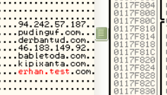The IP-address of the sinkhole hardcoded in the Vawtrak binary

Sinkhole Framework

Modelling and Design

Inventory

I started capturing the traffic with tcpdump from October 2014 on storing all HTTP requests destined to the sinkhole. The complete size of all PCAP files is around 60 GB which is a reasonable amount of data for further scientific research.

The files were split in 50 MB parts and stored on a raw disk image because larger files freeze my system. This also allows me to use the disk in my virtual machines which are used in the implementation phase.

Database Structure

All available information is stored within the PCAP files. It is not possible to search for specific requests or metadata without going through each file. Doing this would take an enormous amount of time for the statistics. Instead I will parse the files, pick all relevant information and store them into a database. This will allow me to do faster lookups and queries for the data.

The database tables can be classified into those which store information from the PCAPs and those which store the results of statistic calculations. These tables are defined in two applications called reportparser and stats.

Reportparser Tables

I will first describe the tables and fields in the reportparser application. The first table is the Bots table which stores the unique bot_id, a pointer to the User-Agents table and a field for the country-code. When a bot sends a request, the header also contains the User-Agent. Multiple bots can have the same User-Agent so I save every unique one in a different table and point to it instead of just saving it in a Bots entry. The country-code will be used for the interface to show where the bot comes from.

Every bot is part of a project which divides the botnet in several sub-botnets. Depending on the project, bots receive different configurations and commands. To see which bot belongs to which project I created the table Projects which stores the project_id and a list of all bots which are part of it.

When a bot comes online it usually sends a Type:00 package every minute to ask the C&C server for new configurations and commands. For the statistics, I need to know when a bot was online, from which IP-address it connected from and how long it was online. For this I designed a session system which starts a session as soon as a bot comes online and refreshes it when the bot sends a request again within a short time range. The session table has a field which points to the Bots table, the IP-address during that session and a timestamp to see when the session starts and ends.

The most valuable data for the botnet operators are the reports. These contain POST-values from forms, full copies of a page or files that are grabbed by the credentials stealer. Bots send reports in encrypted form so I need to decrypt them first and save the data into the database. Both the de- and encrypted form is saved and depending on the type also the URI or pointer to the file on disk.

Beside those tables, I also created the Useragents and IPs table. The table Useragents, which is pointed at by a bot entry, contains the User-Agent string, and fields for browser and operating system information. These will be filled after parsing the User-Agent with a third party tool. It is done similarly with the IP-addresses. There I have the IP-address and fill the other fields like country code and country name by doing GeoIP lookups.

Statistic Tables

The next tables are part of the stats application and will be used for statistic results. On my initial tests I always calculated the statistics on runtime at each request. This was not a good solution as the processing time was getting longer with the amount of data in the system. Instead of doing it on each request, I do the calculations only once and save the results in the corresponding tables. This way I will only need to query the results instead and save time.

I first had to think about which statistics are relevant and which ones could be derived from the data available. The first thing that interests me is the size of the botnet and how many infections and disinfections occur per day. For me an infection is at the day where I see a particular bot for the first time and a disinfection at the day the bot has been last seen. For each case I just need to save the specific date and the amount for each day.

These information are good for getting an overview of the botnet but there are more statistics possible with the data. I also want to analyze meta information of the bots like the browser and operating system they use or where they are located. Information about the browser and operating system will be derived from the User-Agent string and the statistics will show the distribution of vendors and versions.

I will do two statistics for each category because one bot can have multiple User-Agents and there might be a difference if you look at all User-Agents or just at the User-Agent that was used the most by a bot. The first statistic will use the most seen User-Agent of a bot for the calculation and the other one will go through all User-Agents in the system instead. The tables that store the results relative to the bots will be appended by _rel in the table name.

The same principle will be used for the country statistics. Most bots have multiple sessions and IP-addresses associated to them so I will do one statistic looking at all IPs in the system and one where I will just use the most common location of the bot instead.

I also want to see where the bots of each project are coming from. This way it might be possible to see if a particular project targets specific countries.

These statistics should give the scientific community a good understanding and overview of Vawtrak. Table statsmodels shows the tables where the results will be stored after calculation.

PCAP Parser

Processing all PCAP files from the inventory will be the main task of the PCAP-parser. The goal of it is to parse the files in a way so that I am later able to access all data easier and faster for further analysis.

I will now briefly describe the steps involved in this process but the complete implementation will be discussed in the Implementation chapter. The targets of my parser are the HTTP requests which are stored in the PCAP files. For each request it should check if this package is relevant by validating the request URI and pick information like the bot_id out of it. If this bot has never sent a request before then it should be added to the database. The parser will create a new session or refresh the last one if the last request was at most 30 minutes ago.

As there are different kind of reports it should check for the type of it and then treat it differently. If the report contains POST-data then the parser should save the decrypted data in the specific Reports table entry or if the request contains a file then it should just be saved to the disk. When the parsing of a package is complete then it should continue with the following ones till all packages and files are finished.

During my initial tests with the parser, I saw that the process will take a long time due to the sheer amount of data. To have a better overview of this process I created a table called Dumps which stores the filename and two boolean fields which show if the process has started or finished for this file. This way it is possible to resume the process if a crash occurs.

Implementation

The following chapter presents the implementation phase of my bachelor thesis. I will first describe the backend where the analysis framework is deployed and then continue describing the programmatic aspect of the parser and statistic calculators. In the last part I will demonstrate the web interface where the data and statistics are shown.

Backend

The operating system where the analysis framework is deployed is Debian Jessie running on a KVM hypervisor. During some parsing tests I saw that the memory usage was quite high so I gave 8 GB RAM to the guest system and chose 100 GB for the disk image as I was not sure how large the SQL database would get. The database is an instance of PostgreSQL as I had good experience with the performance in other setups.

The analysis framework is build with the Django web framework. Django is a python based web framework using the Model-View-Controller principle thus allowing rapid development of web based applications. Basically all parts beside the documentation of this project are done with Django.

In the following sections, I will first describe the reportparser application and show the detailed steps involved in this process and how I implemented my ideas from the chapter Modelling.

Reportparser

Every Django project contains a file that is called manage.py which allows to control different aspects of the project like doing database migrations, starting the development web server, creating new applications or running custom commands. To create a custom command you have to create a subfolder "management/commands" in the application folder and put the Python file there containing the code.

PCAP Parser

The PCAP-parser implementation is within the custom command filereports.py which is invoked by running manage.py filereports. I will now describe the steps in this command.

The first part of the program checks if the PCAP file was already parsed or if the process crashed in a previous session. A crash is known in entries where the field started is True but is_parsed is False. In this case the file will be skipped.

# Skip file if already parsed or crashed
if dump.is_parsed:
    print("Dump %s already parsed. Skipping ..." % (file))
    continue
if dump.started:
    print("Dump %s crashed last time. Skipping ..." % (file))
    continue
dump.started = True
dump.save()

After this check, Pyshark is used to open the PCAP files and access attributes of all packages within. The first problem I stumbled upon was that Pyshark has no method to access HTTP request bodies. I solved this problem by accessing the complete TCP data through the data.tcp_reassembled_data method instead which returns a colon separated list of hex values. Knowing that the request header and the body are separated by \r\n, I am able to access the data by splitting the output at that point.

payload_raw = package.data.tcp_reassembled_data
payload = payload_raw.split('0d:0a:0d:0a:')[1].split(":")

Everything after the first 8 bytes of the request body is the encrypted report. To decrypt this data, I use a modified version of James Wyke's decrypter that he released with his paper.

def vawtrak_decrypt(payload):
    decrypted_data =""
    seed = int(''.join(x for x in reversed(payload[:4])),16)
    for payload_byte in payload[8:]:
    next = (0x343fd * seed + 0x269ec3) & 0xffffffff
    seed = next
    key_byte = next >> 0x10
    byte = int(payload_byte,16) ^ (key_byte & 0xff)
    decrypted_data += str(chr(int(byte)))
    return decrypted_data

There is more useful data in the package beside the request body. Pyshark additionally gives access to the User-Agent and URI of the HTTP request, the IP-Address and timestamp.

Parameters like the package type, bot_id and project_id are in the URI of the request. To access these values and to check if the URI has a valid form, I created following Regular Expression and skip this particular package if it does not match.

parameters = re.match(r"http://94.242.57.187/channel/0(?P<type_id>[0-2])/(?P<project_id>[0-9a-f]{8})/(?P<bot_id>[0-9a-f]{8})*", uri)
if not parameters:
    continue
type_id = parameters.group('type_id')
project_id = parameters.group('project_id')
bot_id = parameters.group('bot_id')

From this point on I can start filling the database. In the first step I check if the bot is already stored in the database and create the entry if that is not the case. Django has an easy method for this called get_or_create() which does both at once. The same principle is applied for the User-Agent and project entry. If the bot does not have the User-Agent in his entry, then it will be added to it.

# Check if bot exists in database, or else create
bot, created = Bots.objects.get_or_create(bot_id=bot_id)

# Check if useragent is in DB and add relation to bot
ua_obj, created = Useragents.objects.get_or_create(ua=ua)
if created or not bot.useragent.filter(ua=ua).exists():
    bot.useragent.add(ua_obj)

# Check if project exists, or else create and add bot to project
project, created = Projects.objects.get_or_create(project_id=project_id)
if not bot.project_set.filter(project_id=project.project_id).exists():
    project.bots.add(bot)

Implementation of the session system in the next step was a bit more complicated. Every session entry has the field start and last. The field start shows when the session started and field last when the last request in that session was received. I first query the database for the bots last session. If session is older than 30 minutes then a new one is created or else the previous session is used and the field last set to the current time.

# Longest timeout 30 minutes
time_pre = time - datetime.timedelta(minutes=30)
# Find bot's session that was at least 30m ago
if Sessions.objects.filter(bot=bot,last__lte=time,last__gte=time_pre).order_by('-last').exists():
    session = Sessions.objects.filter(bot=bot,last__lte=time,last__gte=time_pre).order_by('-last')[0]
    session.last = time
    session.save()
else:
    # Create new session for this bot
    ip, created = IPs.objects.get_or_create(ip=ip_addr)
    session = Sessions.objects.create(bot=bot,ip=ip,start=time,last=time)

There are different types of reports. Depending on this type the parser processes the report in different ways.

A Type 01 report contains the URI and POST-values that a victim sent to a website. The URI is located in the second line of the decrypted report and the POST-values in following lines. I use a Regular Expression to extract these values. They are stored together with the decrypted body, timestamp, project and session in the database. In case the output of the decryption algorithm is not readable, the data is still stored in a different entry for future use and debugging.

if type_id == '1':
    # Get URI and POST-values from request
    reportpackage = re.match(r"(?P<botprojid>[0-9A-F]{17})\r\n(?P<post_url>http[s]?://(?:[a-zA-Z]|[0-9]|[$-_@.&+]|[!*\(\),]|(?:%[0-9a-fA-F][0-9a-fA-F]))+)\r\n(?P<post_data>(.|\n|\r\n)*)",data_field)
    # Check if valid package
    if reportpackage:
        Reports.objects.create(session=session,project=project,uri=reportpackage.group('post_url'),time=time,data=reportpackage.group('post_data'))
    # If not valid then store in data_invalid instead
    else:
        Reports.objects.create(session=session,project=project,uri=uri,time=time,data_invalid=data_field,data_raw=payload_raw)

Another type is the Type 02 report which has two additional subtypes. These reports contain aPlib compressed files in the decrypted body. The processing of these reports is nearly identical but instead of saving the form data, the parser saves the compressed file to disk. Depending on the subtype, the filename is appended by .html.ap32 (Subtype 5) or .bin.ap32 (Subtype 7).

A code snippet for subtype 5 is shown here:

# Create fileobject with decrypted content
f = ContentFile(reportpackage.group('sourcecode'))
# Create entry in DB for report
rep = Reports.objects.create(session=session,project=project,uri=reportpackage.group('post_url'),time=time,data_raw=payload_raw)
# Add file to this entry and save on disk
rep.data_file.save(bot_id+"-5-"+randomword(16)+".html.ap32",f, save=True)

The parsing process is finished for this particular package and the parser will continue with all the remaining ones. When all packages of a PCAP file are finished the is_parsed field is set to True.

User-Agent Parser

Before I can start doing the statistics, I need to fill additional fields in the table Useragents. For this, I use the Python library user-agents which allows to identify the browser and operating system by parsing the User-Agent.

# Get all UA that are not parsed
ua_objs = Useragents.objects.filter(bfam='',osfam='')
for ua in ua_objs:
    # Parse UA and save values in entry
    user_agent = parse(ua.ua)
    ua.bfam=user_agent.browser.family
    [...]
    ua.save()

GeoIP Lookups

The table Sessions points to the table IPs where all IP-Addresses are stored. By doing GeoIP lookups on these, I am able to tell the approximate location of a bot. I use the library pygeoip and the GeoLite Legacy database to get values like country code and city which are used for the statistics later on.

# Get IP-addresses that are not parsed
ip_objs = IPs.objects.filter(ccode='')

for ip_obj in ip_objs:
    # Parse IP
    record = gi.record_by_addr(ip_obj.ip)
    if record is not None:
        # Store the parsed values to the database
        ip_obj.ccode = record['country_code']
        [...]
        ip_obj.save()

Statistics

After the data is stored to the database I can start doing the statistics. There are different statistics that needed to be done and in these following sections I am going to show their implementation.

Bots Per Day, Infections, Disinfections

The first thing I want to show are the implementations that calculate the amount of bots online per day, new infections and disinfections. These three statistics are quite similar in their implementation so I describe them together in this section.

Determining the amount of bots online per day is not difficult because of the session system which shows when a bot was online. My first approach was to check each day since traffic has been captured and count the amount of bots, but I discarded this idea because there have been days where I have not captured any requests at all due to technical difficulties explained in chapter Results.

So instead, I first determine days where any bots have been online at all and add these dates to a list. Then I search for all bots that have started a session on each of these days and count them. The resulting date and amount is then saved to the database and can be presented in the interface.

sessions = Sessions.objects.all()
dates = []
for session in sessions:
    # Add new dates to the list
    if session.start.date() not in dates:
        dates.append(session.start.date())
for date in dates:
    date_range = (
        # The start_date with the minimum possible time
        datetime.combine(date, datetime.min.time()),
        # The start_date with the maximum possible time         datetime.combine(date, datetime.max.time())
    )
    # Find all Bots who started a sesion on that day and save result
    s = Sessions.objects.filter(start__range=date_range).values('bot').distinct()
    amount = s.count()
    Bots_per_day.objects.get_or_create(date=date,amount=amount)

The next statistics are the infections and disinfections per day and are created in the same process. As a definition, I define that an infection is the day when a bot was first seen and a disinfection the day it was last seen.

The first step involves fetching a bots first and last session. This is done by ordering the session results by the first and last field. Then I iterate the field amount in the results for that day. This way I get the total amount of bots infected and disinfected for each day.

for bot in Bots.objects.all():
    # Get first session
    s = bot.sessions_set.order_by('start')[0]
    # Get last session
    s2 = bot.sessions_set.order_by('-last')[0]
    day, c = Infections_per_day.objects.get_or_create(date=s.start)
    day2, c = Desinfections.objects.get_or_create(date=s2.last)
    # Iterate the amount of infections at that day
    day.amount += 1
    day.save()
    # Iterate the amount of disinfections at that day
    day2.amount += 1
    day2.save()

User-Agent Related Statistics

The next statistics that I implement will show what browser and operating systems the bots use.

I will do two kind of statistics here. The first one will do the calculation for all available User-Agents and the other one will only use the most common User-Agent of each bot. Both calculations are done in the same management command to save time.

The program fetches all User-Agents, gets the browser family and increments the counter for it in the results table Browser. The browser family is also added to a Python helper function called Counter(). When all User-Agents are done, the function most_common of Counter() is used to return the most common browser of a bot which is then used for the incrementation in Browser_rel.

The following listing shows the shortened version of the implementation:

for bot in bots:
    cnt = Counter()
    bot_uas = bot.useragent.all()
    for ua in bot_uas:
        # iterate to get the most common useragent of bot
        cnt[ua.bfam] += 1
        browser, c = Browser.objects.get_or_create(bfam=ua.bfam)
        # Results for counting each User-Agent
        browser.amount += 1
        browser.save()
    bfam = cnt.most_common(2)[0][0]
    # Results for counting most common UA of each bot
    browser, c = Browser_rel.objects.get_or_create(bfam=bfam)
    browser.amount += 1
    browser.save()

Calculations for the operating system are done in the same way, so I will skip the description of that process.

It is also possible to get the architecture of a operating system through the User-Agent string. This is not completely accurate as a x64 operating system can also run x86 browsers. Nevertheless it is at least accurate to say that the operating system is x64 when the User-Agent contains "Win64", "x64" or "WOW64".

After checking for these substrings, the calculations are done in the same way as before and results saved into the database.

IP-address Related Statistics

It is also interesting to know in which countries the bots are located. For the implementation of this statistic I use the table IPs which contains the country name and code for each IP-address.

I do two statistics again depending if the calculation uses all IP-addresses in the system (Table Country) or only the most common country of a bot (Table Country_rel). The calculation is similar to the way it is done for browsers and operating systems.

Beside seeing the absolute world wide distribution of the bots, it is also interesting to see the distributions depending on a project. This way it is possible to guess if a project targets specific countries.

The table Projects has a field bots which lists all bots of a project. For each bot in a project I fetch the field country and iterate count of this country-project combination. The results are saved in the table Proj_Country_Dist.

projects = Projects.objects.all()
for project in projects:
    bots = project.bots.all()
    for bot in bots:
        # Find out the country of the bot and increment the amount in the results
        country, c = Proj_Country_Dist.objects.get_or_create(country=bot.country,project=project)
        country.count += 1
        country.save()

Frontend

The final important part of the analysis framework is the frontend implementation which is used to show all data and visualize statistic results.

Creating a new web interface can become a time consuming task. To speed this up I am using the CSS framework Bootstrap and the free template SB Admin 2 as a base. This way it is possible to quickly implement pages as Bootstrap offers many different components.

Having an intuitive interface is important to find information I am looking for. Its main goals are showing the statistic results and all other information about bots and projects. The following sections will demonstrate the important parts of this interface and describe how different aspects were implemented.

Management

The management area is part of the interface where you are able to see bot and project information. I created overview pages for both cases. The bot overview lists all bots showing the bot_id, country of origin and project.

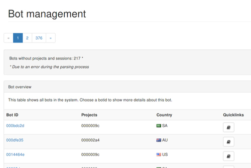Bot overview listing all bots.

You can click on the bot_id to get more detailed information about it. The detail page shows all locations that were found with GeoIP on a map and lists User-Agents and sessions in tables. To display the map, I use the JavaScript library jVectorMap which allows the map to be displayed cross-plattform. Accessing the reports of a bot is also possible by following the Reports link which shows an overview of them displaying the URL and POST-data.

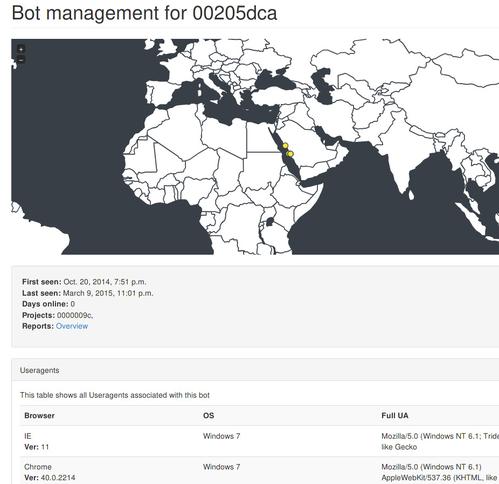Bot detail showing location, User-Agents and sessions.

The projects overview lists all projects and amount of bots that are part of them.

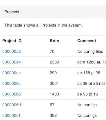Project overview listing projects and amount of bots.

You can see a detail page of a project again by clicking on the project_id in the overview. This detail page lists all bots of this project and a heatmap showing where the bots are from. With this I can guess if a project is targeted for specific countries.

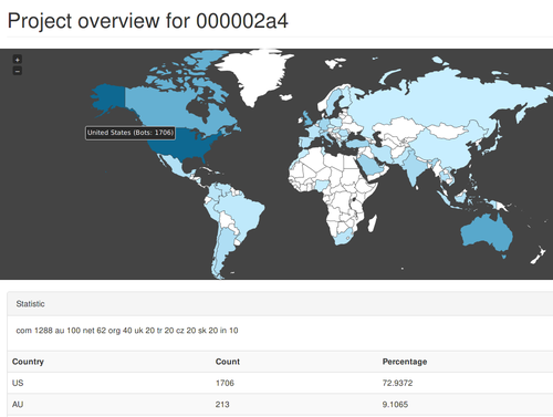Project overview of a single project.

Analytics

In this section, I am going to present the category Analytics and describe the tools I used to visualize the results of my statistics. Depending on the statistics, I use different ways to visualize the data.

The bots per day, infections and disinfections statistics show the amount of bots for each day. The best way to represent this information is by plotting a graph using the data from a specified time range. There are two fields on the page where you can enter a start and an end date to only show the results in this time range.

For the visualization, I use the JavaScript library morris.js which allows to plot data in graphs and charts. The data is queried from the database which means that it is displayed dynamically.

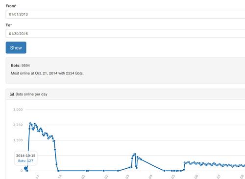Plotting the amount of bots online per day.

The infections and disinfections page looks completely the same, just with differing results from these statistics.

Another statistic is the country analysis which shows the locations of all bots. With this statistic, I have three ways of representing the data. The first way is by using a heatmap of the world using jVectorMap. It shows each country in the world and colors them in a darker blue tone the more bots are from this country. By hovering over a country, you can also see the number of bots.

After that, I use bar charts (morris.js) and display the top ten most common countries in the botnet. I only show the top ten because there are over 90 different countries and it would not fit in the screen. To display all countries, I put a table below the bar chart instead which lists all countries, the amount and a percentage value. This way, these information do not get lost.

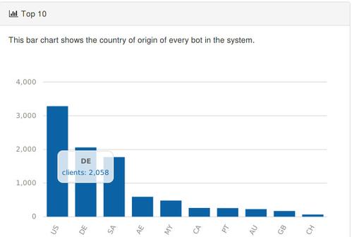Bar graph showing the top ten bot ountries.

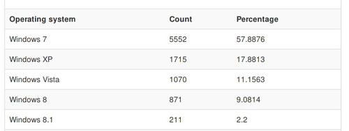
The last statistic in the Analytics category presents the results for browser, operating system and architecture. These results contain the name, amount and a percentage share of the total amount. Displaying these three statistics are done in the same way.

Plotting a graph with these values makes no sense and I display the results in bar charts instead. This way it is possible to see the relations between results on first look. To display all result details, a table is used to show also the percentage share of the total amount.

Bar graph showing the os architectures of the bots.

Results

In the following chapter, I want to present the statistic results and explain their meaning. The first thing I will show are the botnet projects and then continue with the telemetry and statistics derived from metadata like User-Agents and IP-addresses.

Before I can show my results, I first need to talk about a major problem during the capture process that affected the results.

Limitations

I used tcpdump to capture the sinkholes traffic and set a filter to only save packages that go through default HTTP port (80). Before a HTTP connection can be established, there first needs to be a TCP connection. There have been times during the project where I had no tcpdump running. When bots sent reports, they were not saved. The only information that is available from that time is the source IP-address and useragent from the logs.

Therefore, the data is missing in the telemetry statistics and affects the infections and disinfections statistics which I will describe in the following sections.

Projects

The Vawtrak botnet can be divided in several sub-botnets which are called Projects. The table shows all those that were seen during the time of traffic capture.

There are bots in the database that have no project associated to them because of the way the reportparser is implemented. It only saves the project of a bot when it receives a report other than Type:00.

There are 14 different projects that contacted the sinkhole. Four of these projects have the largest share with 8262 of 9421 bots. The largest project 0000009c has nearly a third of all bots with 3051. Most of them are located in Western Asia areas with Saudia Arabia (55%) and the United Arabian Emirates (19%).

James Wyke showed me configuration files for this project that the former C&C have send and these contain target websites with the Top-Level-Domains sa, ae and my*. In my opinion, the combination of these two results proof that the project controllers were successful in targeting these countries.

The next project is 000002a4 which consists of 2339 bots. The bots in this project are from different locations compared to 0000009c. Most of the bots are from the United States (73%) and following to that Australia (9%). The large difference shows that this project is more targeted towards the US. It is interesting to note that all top three targets are english speaking countries.

Defining the target becomes easier with the next two projects 0000006e and 000000b6. These have 1439 and 1433 bots respectively. The interesting thing to see here is that nearly all bots of these projects target a single country. Project 0000006e targets the United States (97%) and project 000000b6 targets Germany (97%) and the rest of the countries are below 1%. The captured configuration files further verify that these countries are actually targeted.

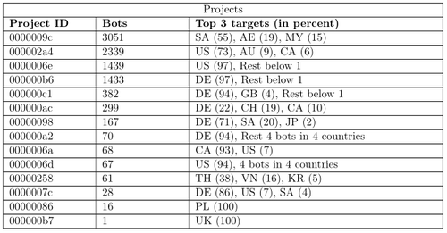Table showing all projects and the amount of bots in it.

Bots Online Per Day

In this section, I will show the statistic results showing how many bots have been online each day during the time of traffic capture. There are only days shown where the capture has been running for a full day. This is because bots are missing if I start the process at 10 pm for example which would affect the statistic.

The first thing I want to note is that here have been 9594 unique bots that contacted the sinkhole and most of them have been online on the 22nd October of 2014 with 2334 bots.

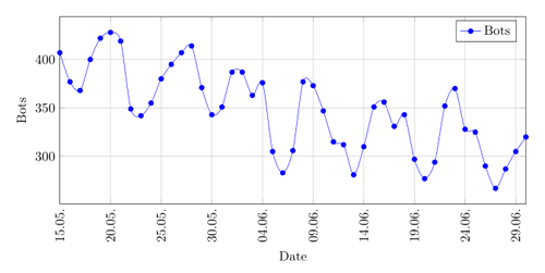
The graph in the figure shows how many bots have been online in the last quarter of the year 2014. In the first days have been more than 2000 unique bots online but it is already easy to see that the amount is decreasing over time. At the end of November, the amount already passed 1500.

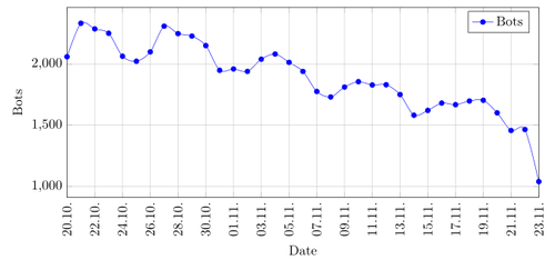Graph showing the amount of bots online per day in the fourth quarter of 2014.

The graph shows a wave like pattern during a week. There are lows on 25.10, 01.11 and 08.11 which are Saturdays. This means that the victims use their computer less on weekends or that some of them are part of companies and not get used. This observation is throughout till the third quarter of 2015.

In March 2015, there are already less bots online with 600 to 800 per day. The time before March is where tcpdump was not running.

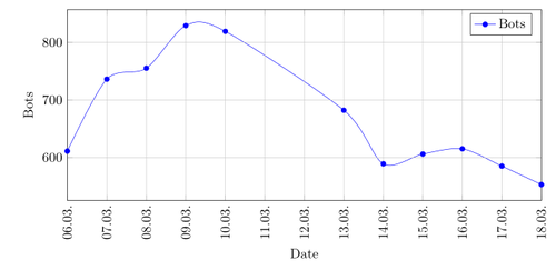Graph showing the amount of bots online per day in the first quarter of 2015.

The second and third quarter of 2015 show the further decline in size of the botnet. In the second quarter there are only between 300 to 400 bots online and in the third quarter only 200 to 250.

The reduction in size is explainable by the fact that victims may use Anti-Virus products or by new setups of their operating system. On the 11th August of 2015 Microsoft released new definitions for their Malicious Software Removal Tool to detect Vawtrak. I expected to see a large drop in the amount of bots per day after that, but there was actually no difference in the trend. This could be due to the fact that MSRT is not deployed on all systems or that the victims do not often update Windows.

Graph showing the amount of bots online per day in the second quarter of 2015.

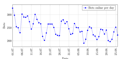Graph showing the amount of bots online per day in the third quarter of 2015.

Infections and Disinfections

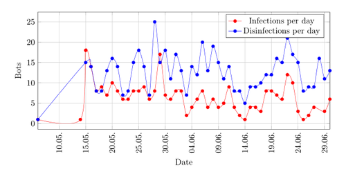
The previous statistic showed already a decline in the size of the botnet. In this section I will show how many bots are newly infected and how many disinfected. There are four figures, each showing two graphs where the red one represents the infections and blue one the disinfections.

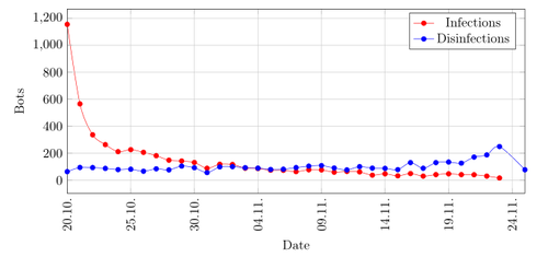Graph showing the amount of infections and disinfections per day in the fourth quarter of 2014.

In the first quarter of 2014 there is a spike at the beginning. This spike is due to the fact that an infection is defined as the first time a bot contacted the sinkhole. On the next days less new infections happened and on third November 2014 there are the first time more disinfections than infections. The disinfections stay quite stable at around 100 per day and spike a bit towards the end of November. This is for the same reason as described with the infections before. All bots that are disinfected between 24th November of 2014 and first March 2015 are added before the 24th November depending when they send a request the last time.

Graph showing the amount of infections and disinfections per day in the first quarter of 2015.

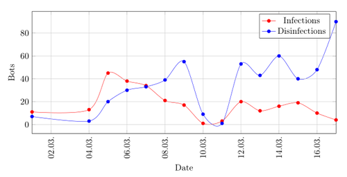
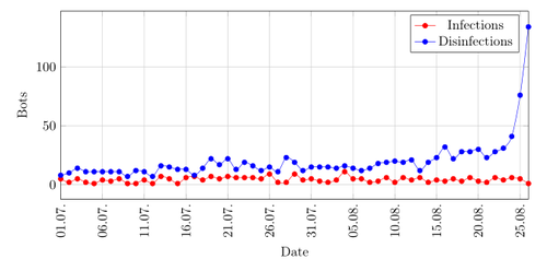
Graph showing the amount of infections per day in the second quarter of 2015.

The first two quarters of 2015 show a drop in infections and disinfections and you can see that there are nearly always more disinfections than infections which explains the reduction of the botnet size. The numbers of new infections are very low and not coming near ten in the third quarter of 2015. It was a bit unexpected to see new infections towards the end, because it is logical to assume that the malware authors would not add an IP-address which they do not control anymore. The reason for new infections may be because older versions of the malware are still circulating on the internet.

Graph showing the amount of infections and disinfections per day in the third quarter of 2015.

Locations

In this section, I will present the country analysis results that show in which countries the bots are located. The bots are located in 92 different countries but I will only show the ten most common ones.

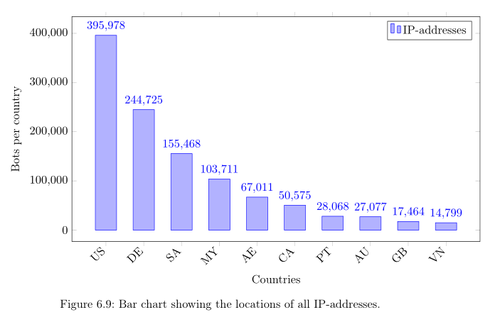Bar chart showing the locations of all IP-addresses.

The first analysis is based on all IP-addresses in the system. Here we can see that the most IP-addresses are from the United-States (395,978), Germany (244,725), Saudi Arabia (155,468) and Malaysia (103,711). The problem with this statistic is that the results are affected depending if a particular country uses more dynamic or static IP-addresses. A country with more dynamic addresses will have higher values than a country that uses static addresses.

To bypass this problem and have a better representation of the situation, I had to determine the country of a bot. As described in the implementation chapter the most likely country is defined by the most common location of a bot's IP-addresses. The results of this statistic is shown in the figure. Here you can see that the most bots are again from the United States (3,282), Germany (2,058) and Saudi Arabia (1,700). Malaysia and the United Arabian Emirates switched ranks in the list due to the dynamic and static IP-addresses.

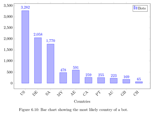Bar chart showing the most likely country of a bot.

Browser Vendors

After the telemetry statistic, I will now present statistics on meta information of the bots. The reference for these statistics is the User-Agent and I will begin showing the distribution of browser vendors.

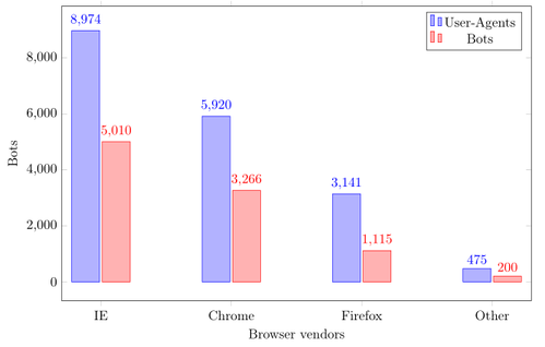Bar chart showing the distribution of browser vendors.

There are two different results in the bar chart in the figure. For the blue bars all User-Agents were used for the calculation and for the red one only a bot's most common User-Agent.

The first thing to see here is that the relations of the results are quite similar. Internet Explorer is ranked first here, followed by Chrome and Firefox. The reason why Internet Explorer is first is explainable by the fact that it is the default pre-installed browser in Windows. Chrome and Firefox can be manually installed but there is a clear tendency towards Chrome (3,266 bots) instead of Firefox (1,115).

The element Other contains User-Agents that could not be parsed and also User-Agents like wget which were maybe used by other researchers.

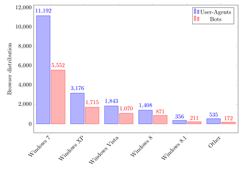
Operating System

Vawtrak is a malware family that runs only on Windows. In the operating system statistics we will see which versions of Windows the bots use.

In this statistic, I also have two results in the same way as it was shown in the browser statistic. The blue bar shows the results of all User-Agents again and the red one the results of a bot's most common one. Leaving out Other, the ranking for both cases is the same.

{: .img-luid .rounded .mx-auto .d-block} Bar chart showing the distribution of operating systems.

Windows 7 is the most used operating system with more than 50%. Following that is Windows XP with 18% even though Microsoft ended Support for XP April 2014. In my opinion this shows that the victims may not be tech-savvy.

The amount of Windows Vista bots and Windows 8 (including 8.1) is nearly similar at 11%. Some of the User-Agents I saw in other were actually Windows 10 machines but the parser did not detect these. This shows that Vawtrak is compatible with Windows 10.

OS Architecture

The last thing I am going to present is the architecture analysis. It shows how many bots use x86 and how many x64 systems. The result for the x64 systems is the minimum value as this was derived from strings in the User-Agent which hint towards x64 systems.

Here we see that at least one third of the bots is using a x64 Windows system.

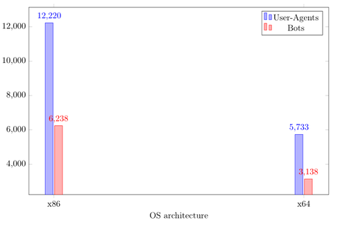Bar chart showing the distribution of operating system architectures.

Conclusion

Vawtrak is a sophisticated banking Trojan for Windows. In this project, I have implemented an analysis framework which is able to parse captured traffic of Vawtrak C&C servers and create statistics about the bots contacting them. Implementing the network protocol was easy due to the already released scientific literature from the AV industry.

I have captured 60 GB of traffic from a Vawtrak sinkhole and parsed the data in the analysis framework. After that, I created the statistics which are derived from the bot's User-Agents and IP-addresses.

A total amount of 9594 bots contacted the sinkhole from October 2014 to August 2015 of which most are located in the United States (34%), Germany (21%) and Saudi Arabia (18%). The most common operating system is Windows 7 (58%) and the most common browser Internet Explorer (52%).

Taking down the botnet by shutting down the C&C servers is not advisable as any arbitrary person could get the IP-address by chance like it was in my case. With the scientific literature it is then easily possible to get back control of the bots.

Due to legal reasons, a takedown should not be done by private persons but instead only by legal authorities in cooperation with researchers.

I propose that a takedown should be done in two phases. The first phase should be a one week long observation where traffic of the C&C servers is captured passively. This way it is possible to estimate the size of the botnet.

In the second phase the traffic of all C&C servers should be redirected to a server which only responds with a disinfect command, removing the malware from the victim's system. This is still possible at the moment because the authenticity of the commands is not cryptographically checked.

Solving the problem on client side may allow to finally take down Vawtrak. This operation may be an unique opportunity as it is most likely that the operators behind Vawtrak will add digital signatures to their commands in the future.

At last I want to thank especially Horgh and James Wyke (FireEye) for all their help during this project. Without you guys, this would not have been possible.